On Some Aspects of Low-Noise Electronics Design

​Low-noise equipment finds many uses: in satellite communications, radars, radio astronomy, and precision measurement instruments. Let’s consider two engineering tasks from our own embedded hardware design practice. These examples come from very different domains: high-fidelity audio systems and medical diagnostics. The first task requires amplifying the signal from a moving coil phono cartridge. The second one requires boosting brain bioelectric potential.

The Integra team has successfully tackled engineering challenges across diverse fields from consumer electronics to industrial and medical solutions. If you’re planning to  design low-noise electronics or other types of custom hardware, contact our team for a consultation.

​Though the tasks mentioned earlier appear unrelated at first glance, both demand high-quality amplification of extremely weak signals that can easily get lost in the amplifier's internal noise. So, if we ignore the amplifier's own noise during electronics design, it can result in a non-functional device.

Let’s start off with several common noise types that engineers frequently address when dealing with low-noise electronics design.

Types of Internal Noise

Thermal Noise

Thermal noise, or Johnson noise, is a random noise voltage that arises from the random thermal motion of particles in the resistive element.

Any component with non-zero ohmic resistance generates this noise as long as its temperature is above absolute zero (-273.15°C). Even a resistor that is simply sitting on a workbench acts as a thermal noise generator. Thermal noise is white noise, meaning it has a flat frequency spectrum. The formula below gives the root-mean-square (RMS) noise voltage generated by a resistor of value R at temperature T over a bandwidth 𝚫ƒ and measured in V(rms).

Here is another formula that shows the spectral density of thermal noise voltage, measured in $V(rms)/\sqrt{Hz}$.

One can use a simplified version that omits Boltzmann constant. The result is measured in $nV/\sqrt{Hz}$:

For example, a 1 kΩ resistor at room temperature has noise voltage spectral density of 4.1 $nV/\sqrt{Hz}$. It generates 581.2 nV(rms) in a 20 kHz audio bandwidth.

Shot Noise

Electric current is an ordered flow of charged particles, i.e., it has a discrete nature. As a result, a steady-state DC current value shows fluctuations. This is shot noise, or Poisson noise. It’s another example of white noise with a flat spectrum.

The formula below gives the (RMS) noise current for a DC current I_dc over a bandwidth 𝚫ƒ measured in A(rms).

The formula for noise current spectral density measured in $A/\sqrt{Hz}$ is as follows:

We can also use a handy simplified version that gives a value measured in $pA/\sqrt{Hz}$:

Important note: these formulas apply only when charged particles penetrate an energy barrier—for instance, a diode's p-n junction or a bipolar transistor's base-emitter junction. The current in purely resistive circuits generates far less shot noise.

For example, a transistor base current of 10 μA produces noise current density of 1.78 $pA/\sqrt{Hz}$. That's 251.7 pA(rms) in a 20 kHz audio bandwidth. It might seem tiny, but as we'll see later, you can't always ignore these levels.

Flicker Noise

Flicker noise, or 1/f noise, is extra electronic noise stemming from irregularities in the conductive material, as well as from charge carrier generation and recombination in semiconductors. It has a pink spectrum, where power drops as frequency rises.

Noise types covered above are irremovable due to fundamental physics. For instance, even top-tier, pricey resistors produce the same thermal noise as cheap carbon ones of the same value. On top of that, in real components, there are sources of additional noise. Actual components have resistance fluctuations that create additional noise voltage proportional to the DC current flowing through. It’s a classic case of flicker noise in components.

The graph below shows noise voltage spectral density versus frequency, with a clear flicker component. You can see the corner frequency that roughly separates pink and white noise regions. The lower the corner frequency, the better the component's noise performance.

Now let's cover the key parameters to consider when designing low-noise electronics.

Signal-to-Noise Ratio (SNR)

It is the ratio between signal power and noise power typically measured in decibels. You can express it using signal and noise powers:

Or via their RMS voltage values:

Keep in mind that for narrowband signals (e.g., a single tone), widening the measurement bandwidth hurts SNR, since noise power rises while signal power stays the same. The goal is always to maximize signal-to-noise ratio.

Amplifier Noise Figure (NF)

It is the ratio between the output signal of an actual amplifier and the output signal of an ideal, noiseless amplifier with the same gain and source resistance R_s at the input. Amplifier noise figure is measured in decibels. While SNR describes the signal, ANF describes the amplifier itself. It shows how much the real amplifier's noise affects the overall circuit noise, or, put another way, how much noise the amplifier produces compared to the noise from source resistance.

This also means that there is no point chasing an ultra-quite amplifier for a source with high internal resistance: the source's own resistance noise will still corrupt the signal. 

There are two ways to calculate amplifier NF—by using noise power or the ratio between input and output SNR:

Ideally, the amplifier noise figure should equal zero, so engineers should aim for this value.

For example, a circuit with an LM358 operational amplifier, whose noise voltage spectral density equals 40 $nV/\sqrt{Hz}$, will have an amplifier noise figure of 30 dB when working with a 100 Ω source. Replace the op-amp with an OP27, whose noise voltage spectral density equals 3.5 $nV/\sqrt{Hz}$, and the noise figure drops to 11 dB. As we will show below, an acceptable noise figure here is less than 3 dB, so neither option is really suitable for this source.

Amplifier Noise Model

Amplifier noise can be easily described with the simple model below which is accurate enough for most practical uses.

The noise voltage source (e_n) adds noise voltage to the useful signal, while the noise current source (i_n) causes a noise voltage crop across the signal source resistance (R_s). The drop also adds to the useful signal the same way e_n does. To calculate the total contribution of both noise sources, add their power values, i.e., calculate their root of sum-of-squares. You can see the equation for the total noise voltage e_a measured in $V/\sqrt{Hz}$ below:

This model enables precise noise prediction and circuit optimization. If you're facing challenges related to processing weak signals due to internal noise, contact Integra Sources for assistance with calculations and prototyping.

Examples of Low-Noise Circuits

Let's circle back to the challenges mentioned in the article introduction and see how to apply the described concepts in real electronics designs. The tasks are to develop a preamplifier for a moving-coil phono cartridge and one for EEG diagnostics. Both examples are drawn from Integra Sources’ actual projects, but here we will use simplified schematics for clarity.

MC Phono Cartridge Preamp

We shall start with analyzing the signal source as the first step. The cartridge coil has very low resistance (around 10 Ω) and outputs a tiny signal (about 500 μV). To identify the required noise performance of the amplifier, we need to take into account that a typical vinyl dynamic range is about 70 dB. In other words, the quietest signals that can be recorded on a vinyl are 70 dB below 500 μV, or roughly 160 nV. Hence, the preamp's noise voltage in the audio band must stay below that.

After dividing 160 nV by the square root of the 20 kHz audio bandwidth, we get 1.1 $nV/\sqrt{Hz}$. This spectral density of noise voltage is sufficient, and it shouldn’t be any higher than that. The spectral density of noise current can be ignored in this particular case due to the low source resistance. Hitting 1.1 $nV/\sqrt{Hz}$ because of noise current alone would require 110 $pA/\sqrt{Hz}$. By comparison, typical noise current spectral density of bipolar op-amps typically range from 0.3 to 2.5 $pA/\sqrt{Hz}$.

Now, let's look at an op-amp-based implementation of the circuit.

We chose the LT1028 op-amp to build this amplifier. It boasts a very low noise voltage of 0.85 $nV/\sqrt{Hz}$, comfortably meeting our 1.1 $nV/\sqrt{Hz}$ target. That said, there's room to optimize the circuit even further.

A discrete preamp circuit design delivers even lower noise. This comes from using ultra-quiet bipolar transistors (Q1 and Q2), that work with high collector currents, in the input stage. Plus, unlike the first circuit, there's no need for an expensive, ultra-low-noise op-amp here. The op-amp (U1) handles signals already boosted by the input stage. The first stage boosts the signal by about 40 times, so the noise contribution of the op-amp decreases by the same factor. The OP27 with 3.5 $nV/\sqrt{Hz}$ used here will contribute about 87 $pV/\sqrt{Hz}$. Even a cheaper and noisier NE5532 would work fine, since spectral densities of noise voltage add as the root of sum-of-squares.

You could also make a simpler discrete circuit by using a single input transistor instead of two. It's cheaper and easier to build, and, what’s more important, it’s quieter. However such a circuit needs around 10,000 μF of capacitance in the feedback loop. 

A few words on noise in bipolar transistors.

Noise voltage in bipolar transistors is shot noise in the collector current, which causes voltage drop across the emitter's dynamic resistance. That means you can get pretty much any reasonable noise voltage level in bipolar transistors just by increasing the collector current. Then why did we pick extremely quiet transistors for this circuit? Bipolar transistors have an important parameter that limits their noise performance—base spreading resistance. The term simply refers to the ohmic resistance of the base region that generates thermal noise. Eventually, pumping more collector current hits diminishing returns, and the transistor's noise is dominated by that base resistance thermal noise.

Bipolar transistors typically have base resistance from tens to a couple hundred Ω. But the ones in this circuit clock in at just 1.7 Ω, letting you increase collector current effectively to cut noise. Here, each transistor runs at 10 mA. For comparison, each transistor in LT1028 runs at 900 μA. Noise current is straightforward: it is tied to base DC current. But beyond the source internal resistance, it also causes voltage drop across the base resistance.

Preamp for EEG Diagnostics

EEG is a niche medical field, and solid public data on signal sources is scarce. That’s why we have to use the source thermal noise with a known resistance to determine the requirements for the signal source and optimize the amplifier's noise figure. 

EEG uses a differential measurement circuit, with each electrode resistance ranging from 1 to 10 kΩ. So, the overall source resistance spans 2 to 20 kΩ. This wide variation stems from natural differences in skin thickness, surface preparation quality, and electrode contact stability. On top of that, we are going to need a low input current amplifier in this application: it's indirectly tied to noise but narrows component choices.

With such high source resistance, amplifier noise current matters a lot. Low source resistance emphasizes noise voltage in the amplifiers' noise figure while high source resistance spotlights noise current. Engineers must strike a balance for all cases, so we mapped the noise figure for the two source resistance extremes.

This lets us nail down recommended preamp noise performance. Here, we chose a maximum allowable noise figure of 3 dB for the amplifier, as this level contributes as much noise as the source resistance itself. For low source resistance, noise voltage dominates. We should keep it under 5.8 $nV/\sqrt{Hz}$ for noise figure below 3 dB. For high source resistance, we can use noise current, which must stay below 0.9 $pA/\sqrt{Hz}$ for the same noise figure of 3 dB. The graph's green zone shows the permissible values region. 

As before, let's first examine an op-amp-based implementation of the circuit.

We selected the OPA2210 op-amp for the circuit. Its bipolar input transistors deliver notably lower noise voltage than FET-based op-amps—2.2 $nV/\sqrt{Hz}$. Low collector current in the input stage, paired with super-beta input transistors, keeps input current to just 300 pA. As a result, the operational amplifier has a tiny noise current of 0.4 $pA/\sqrt{Hz}$.

Here's an interesting detail. If we plug the input current value (300 pA) into the shot noise spectral density formula, we will get 11 $fA/\sqrt{Hz}$. Then why does the datasheet list noise current 36 times higher? The OPA2210 uses a bias current cancellation circuit—the input transistors in the op-amp are biased by the current source that gives them nearly the same current level they need for operation. The uncompensated remnant from process variation is the typical input current, which can even flip polarity.

Note that while this scheme sharply cuts DC input current, it does not reduce the shot noise from that current. In fact, it slightly increases that noise. In other words, one can’t rely on input current value to gauge noise current in op-amp-based circuits.

The circuit delivers solid noise performance for this application. The total noise voltage is 3.3 $nV/\sqrt{Hz}$, and noise current is 0.4 $pA/\sqrt{Hz}$. It's good enough, but we can do even better.

Once again, the discrete circuit preamp design outperforms. This is mainly because  the op-amp version needs two differential stages—one stage inside each op-amp—while the discrete one manages with just one. Fewer input components create less noise.

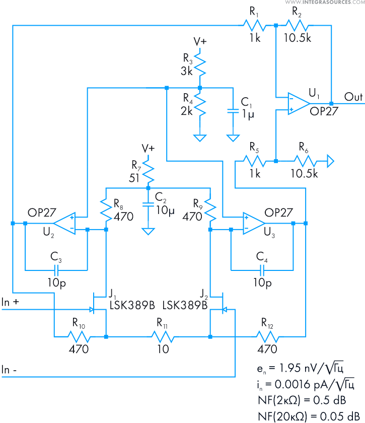
We picked the LSK389 for the input stage. It’s a matched low-noise pair of junction field-effect transistors (JFET). Each delivers 1.3 $nV/\sqrt{Hz}$ noise voltage density. Noise current is negligible: JFET gate input current doesn’t exceed tens of pA, making the corresponding noise current irrelevant for the given source resistances.

A quick note on JFET noise sources: noise voltage stems from channel resistance thermal noise, while noise current is caused by gate leakage current. A powerful transistor generates less noise voltage; lower gate leakage causes less noise current. 

In-House Component Measurements

Before wrapping up, we’d like to share results from internal noise measurements on some components we did in-house. 

Let’s start with the graph of noise voltage versus frequency for bipolar transistors. Collector current was 20 mA during measurements. We can single out two groups here.

The first (bottom seven traces) includes medium- and high-power transistors, most of which are switching type. They were often used in switching regulators back in the day.

They feature low white noise levels thanks to low base spreading resistance. For instance, the quietest here, the 2SC2335, only has 0.2 Ω. But these transistors rarely offer high beta, which is only 25 here. An “amplifier” based on such a device would have too high base current, spiking noise current. There are more interesting compromises, like the FZT851 we saw earlier with beta of around 200 and base spreading resistance of 1.7 Ω, or the 2SC5707 (350 and 2.4 Ω) and 2SC5888 (390 and 3.6 Ω).

The second group (top three lines) comprises low-power transistors. They show mediocre white and 1/f noise but often decent beta. One particularly interesting component is the 2SC1815 from Toshiba designed for audio systems. Its datasheet lists typical base spreading resistance at 50 Ω, and our measurements prove it: the sample hit 53 Ω.

We also measured base current noise for the FZT851. Collector current was 6 mA, while base current was 30 μA during measurement.

Notice how high frequency-wise the corner frequency sits—around 500-600 Hz. That's typical for bipolar transistor noise current, and you'll see the same in bipolar op-amps. 

We did a bit more testing of FET transistors we had in our office. Only the BF245 and LSK389 mentioned above can qualify as quiet. There’s also a fake 2SK170 with high white noise but a decent corner frequency for a JFET. The rest barely suit low-noise electronics design. As for the MOSFET, its corner frequency is way beyond audio band. As you can see, even quiet JFETs have their corner frequency even higher than bipolars.

Finally, let’s take a closer look at 1/f noise in a thick-film SMD resistor. Thick-film resistors suffer from very high flicker noise. The graph below shows noise voltage for an amplifier based on the LSK389 JFET:

The red graph shows the performance of a transistor with thick-film resistors in the drains. The blue graph shows the cheapest metal-film through-hole resistors with a tolerance of 5%. The difference is on the outside. Note that these resistors' noise impact is decreased by about 10 times since they're in the drains of the input transistors. Yet it still strongly impacts the overall circuit noise. So, engineers should stick to thin-film, metal-film, or foil resistors when designing low-noise hardware. 

Conclusion

When designing low-noise electronics, the key task is to achieve the required quality of the useful signal while minimizing the internal noise of the amplifier for a given signal source. In some cases, noise voltage is the dominant factor, in others it is noise current or both these parameters at the same time.

To succeed, it is essential to understand the nature of thermal, shot, and flicker noise, to know how to work with signal-to-noise ratio and amplifier noise figure, and to choose appropriate architectures and components. What counts as “low-noise” will differ between applications: in some projects, op-amps with noise voltage of 10 $nV/\sqrt{Hz}$ are acceptable, while others projects may require no more than 1 $nV/\sqrt{Hz}$. By taking these and other factors into account, engineers can design a circuit that does not drown out a weak signal with its own noise and remains practical to implement in a specific project.

Integra Sources has extensive experience developing not only low-noise electronics but also hardware and software for medical and industrial equipment, agricultural solutions, oil and gas hardware, and more. Contact us if you’d like to receive an expert consultation on your project.