Mathematical Representations of PID Controller Gains

Proportional–integral–derivative controllers, or PID controllers, find many applications. They are used in controllers for BLDC motors, flight controllers, and power factor correction units. You can find dozens of them in electric vehicles. PID controllers are a part of temperature and humidity control systems used in the manufacturing, chemical, and pharmaceutical industries. PID controllers are used in power electronics (particularly in converters), industrial furnaces, and almost all automated processes in manufacturing.

To calculate a control signal, the PID algorithm uses three control terms – proportional, integral, and derivative. Each component is multiplied by a gain that is used to adjust the weight of each term in the equation. This way, engineers can tune a PID controller to suit a particular process. Read our previous article to learn the basics of PID controllers.

The developers in Integra Sources have considerable knowledge and experience with this mechanism. We have successfully used PID controllers in various projects. If your project requires automation as well, PID control may be the most suitable choice. Contact us to consult our team. 

A PID controller can be tuned intuitively, which is one of the key advantages of this mechanism. However, tuning PID controllers is one of the most perplexing topics in engineering. It is not surprising that inexperienced engineers often fail to understand how to tune a controller and adjust the gains. In this copy, we will unravel the issues.

But first, let us turn to history. 

History of PID Controllers

If you try to look for the patent on the world’s first PID controller, you will find none. Back then, PID controllers were not distinguished into separate devices. Instead, engineers gave different names to the tools that performed this function. For instance, the device for automatic course-keeping used on ships was called an “automatic helmsman.” But in fact, it was a type of PID controller.

The most spectacular demonstration of a PID controller was probably the presentation of the airplane autopilot. On June 18, 1914, at an exhibition in France, two pilots climbed on the wings of their plane right in the air to show that the aircraft could fly without manual steering.

The demonstration sparked great interest in autopilots, and PID controllers began to increasingly replace manual control. Companies started to develop different implementations of the PID mechanism. To avoid patent disputes, manufacturers had to modify the devices. Because of varying representations and implementations of the algorithm, customers had to re-educate their staff when migrating from one manufacturer to another. Naturally, this vendor lock-in played into the hands of the manufacturers and did not promote the emergence of a uniform representation.

It is worth noting that the mathematical description of the PID controller was obtained more than 10 years after it was invented. Thus, the device is the result of engineering intuition rather than antecedent mathematical optimization.

Transient Response Performance Indicators 

Before moving on to PID gain calculation, we need to understand what is considered a well-tuned controller and a poorly tuned controller. Certainly, the criteria for each particular system are different. To bring about uniformity, engineers use transient response performance indicators. In this copy, we only talk about the indicators that directly characterize the quality of a transient response because they can be easily seen on a graph. There are also indicators that characterize a transient response indirectly and that need to be calculated, but we will not consider them here. 

Let’s take a look at a hypothetical graph of a transient response to a test step input:

• Settling time

The most useful characteristic here is the settling time. This term refers to the time at which the step response input stays within some small percentage range of the steady-state value (y_final). 

• Process variable

y(t) is the value of the parameter regulated by the controller (process variable). It changes over time as the plant responds to an input (to step response input or new set point).

• Steady-state process value (y_final)

y_final is the process variable value in a steady state. To define when a system reaches a steady state, engineers use a range of values. If the process variable oscillates within this range, then the system is considered to be in a steady state. If the oscillations of the process variable fall outside of this range, it means the transient response isn’t over. Usually, this value range equals +/- 2…5% of the set point on the condition that at the beginning of the transient response, the process variable equals zero. These values are defined for each transient response individually in accordance with the requirements for the system. 

• Overshoot (σ)

The next indicator to which engineers pay attention is overshoot. To measure this value, first we need to define the peak of the process variable (y_max) on the graph. Then, we must make simple calculations:

Thus, overshoot (σ) is the percentage ratio of the maximum deviation of the process variable (Δу_max) to its steady-state value in the direction opposite to its initial deviation. Some systems never cause overshoot. Their transient response can be described as a monotonously increasing function (see the graph below):

The purpose of tuning a PID controller is to minimize the settling time so that the overshoot doesn’t exceed a certain level defined by the requirements for the system. Often, engineers are tasked with eliminating overshoot completely. All these requirements are defined for each system individually. 

• Steady-state error

Steady-state error is another important characteristic of a transient response. It is the difference between the desired process value (set point) and the actual process variable after the plant stabilizes. You can see the steady-state error on the graph below:

An ideal process should not have a steady-state error. However, for a number of reasons, eliminating it isn’t always possible. In that case, engineers strive to minimize it so that it doesn’t exceed a certain value.

The performance of a transient response can be evaluated with other characteristics as well, but these are more common. The requirements for each system are also defined individually. Contact our team and we will help you to get insight into other performance indicators of a transient response and formulate requirements for your system. 

Representations of PID Gains

• Proportional gain

The abbreviation “PID” is derived from the first letters of the multipliers of mathematical functions of addends – the proportional, integral, and derivative terms. Engineers typically use the simplified modification of the PID controller that contains only the proportional term – the so-called P controller (K_p). The preferred term “gain” is sometimes replaced with the term “band.” Band is inversely related to the regular proportional gain, which confuses inexperienced engineers:

• Integral gain

The most essential of the three control terms – and the most confusing one – is probably the integral term. There are two popular but mutually inverse representations of the integral gain. One (K_i) is often used in academic practice while the other (T_i) is more common for engineering practice. They are related by the following equation:

The peculiarity of this gain is that it does not always enhance but often degrades the performance of a transient response. Highly skilled engineers like the ones on our team always have a clear idea of why they use this gain and for what it is needed. It makes us qualified for developing electronics with automated control systems. 

If a controller drives a system to a desired process value with a certain error that will not disappear on its own (steady-state error), this is when the integral term is required. In addition, the Ti gain is proportional to the settling time of the process. That’s why engineers prefer Ti rather than the academic Ki gain. Other than that, adding the integral term increases settling time, overshoot value, and oscillation, as well as decreases gain and phase margin.

• Derivative gain

The representations of the derivative gain have no significant differences and follow the same principle, although they are denoted with different symbols:

When tuning the derivative gain, one should remember that it amplifies noise. Novice engineers usually forget that a mathematical model does not contain noise, unlike a real device. While tuning this gain, engineers should find a compromise between the quality of the transient response and noise sensitivity.

Forms of PID Controller

These are not the only variations here. There are different forms of PID controller representations, which cause confusion, too. When reading an article about how to tune PID gains, pay close attention to the form of the PID equation. Here are the three most popular forms:

Pay attention to the 1^st and 3^rd forms. Let’s see which one is easier to tune. We will use the PI modification for this experiment. We will not use the D term because its behavior in different controller modifications is the same. The 1^st equation is referred to as the parallel form and is often used in the academic environment, while the 3^rd equation is referred to as the series form and is often used by engineers.

Let us plot the diagrams of the direct transient response performance indicators: settling time and overshoot value defined by the gains of the PI controller. In control theory, the Laplace transform is often used to mathematically describe a system. Let’s use a second order as a mathematical model:

This model can describe motor speed (at startup). A similar model would describe the temperature in a chemical reactor.

Now, we connect the PID controller to the plant and close the negative feedback loop.

How PID Gains Affect the Transient Response

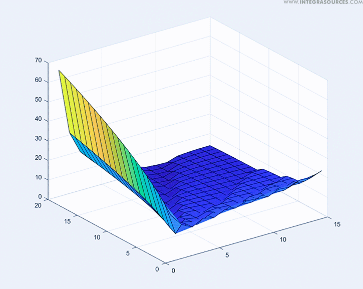
Let’s take a look at the series of surfaces formed by one of the transient response characteristics in function of the integral and proportional gain values. The gain values are indicated in relative values. The proportional gain axis has values from 0 to 40. The integral gain axis has values from 0 to 80. Let us first consider the parallel form and the settling time.

Now, let’s take a look at the behavior of the series form (3^rd):

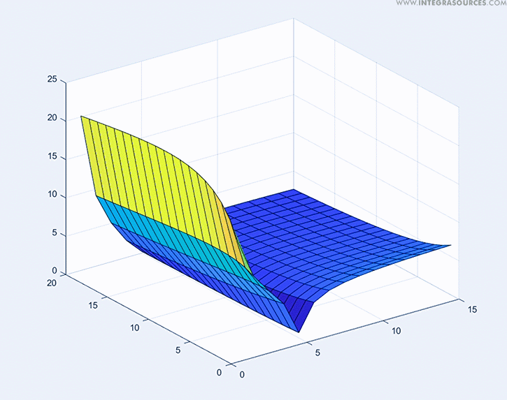
Engineers usually strive to minimize settling time. In other words, the lowest point on the surface corresponds to the minimal settling time of the transient response. The graphs show that the surface of the series form is less steep. It means that tuning the gains becomes more comfortable and smooth, minimizing the chances to miss the most optimal values. The minimum in the series form is more explicit, and the minimum values are parallel to the axis. It makes the tuning process easier as engineers need to adjust only one gain. 

On top of that, in the series form, the deviation of plant parameters from the mathematical model will impact the system dynamics less compared to the parallel form. That is why this form is more popular in practical electronics development.

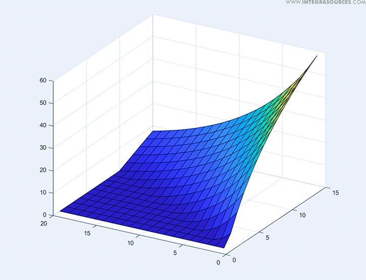
Now, let’s see how PID controller gains affect the overshoot. Similar to the previous case, the surfaces represent the overshoot value in function of the gains:

We shall plot another graph for the series form:

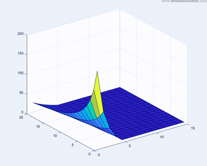
The results are similar, and both surfaces are sloping. However, in the series form, the surface bending is parallel to one of the axes. It makes tuning the controller easier as engineers need to adjust only one gain to achieve the required characteristic in the series form instead of two (required in the parallel form).

Conclusion 

Tuning PID gains is not a simple task for a novice engineer since it requires experience with control loops. The fact that devices use different forms of PID controller representations makes it even more difficult. Tuning a control loop by adjusting gains is a common method in engineering practice. Engineers don’t always have enough time or resources to identify a mathematical model of a plant for subsequent gain calculation. Instead, they typically tune PID controllers with test inputs by changing the set point and watching the system response. Then, they adjust the gain values and repeat the test input. The process goes on until a satisfactory result is achieved. 

As you can see from the surfaces of the settling time and overshoot as functions of the gains, one needs to adjust two gains in the parallel form and only one in the series form to reach the same value. On top of that, the minimum values in the series form are more explicit. These factors make it easier to tune a control loop in the field with the help of test inputs. That’s why the series form of the PID controller is used more commonly for embedded systems. 

But if you have a mathematical model that describes the plant well enough, then the gains can be calculated by one of many methods; for instance, by the Ziegler–Nichols method. In this case, the form of the PID controller makes no difference.

Our company has experienced engineers well familiar with PID controllers. If your business needs automated control systems, feel free to contact our team and discuss your project.